Contents
Related Help Documents
- Data
Selection: Explanation of the program used to select
hybridizations (arrays) for viewing or analyzing data
- Analysis
Methods: Information about the algorithms used for hierarchical
clustering and Self-Organizing Maps (SOMs)
- File
Formats: Information about preclustering (.pcl), clustered data
table (.cdt), gene tree (.gtr) and array tree (.atr) files generated
in the process of clustering data
The Data Selection for Analysis tool is available only after you have
selected a set of hybridized arrays using either the
Basic Search or the
Advanced Search programs.
Once a set has been selected, Data Selection for Analysis allows you
to select genes or spots to cluster, and to filter data based on a
variety of parameters. This tool can be used to generate a
preclustering (.pcl) file, or the files needed for viewing a cluster
with TreeView. In addition, Data Selection for Analysis will lead you
to tools that will let you view clustered data via the web.
Data Selection for Analysis is split into three large steps:
- Gene Selection & Annotation allows
you to choose the genes or spots to retrieve for analysis, how to
represent and annotate the genes and how to describe the hybridized
arrays you've selected.
- Data Filtering Options gives you options for
selecting which data column to retrieve and to filter the data
retrieved based on values of any of the data associated with the
results.
- Gene Filtering Options
allows you to filter genes based on their data as well as to transform
(center) data.
Although we use the word 'gene,' it really refers to any DNA sample
spotted on the microarrays. A 'gene' might be a PCR product
representing an entire section of a gene, a portion of a gene, a clone
associated with a gene, an intergenic region or anything at all.
This section allows you to first specify which genes are of interest to you, then decide
how to collapse your data, how to identify genes in your output file, select biological annotation and to choose a way
to label the arrays you're using.
- Specify genes or clones for which to retrieve results:
Use one of the following three options for deciding which genes on
your arrays for which to retrieve data. Only genes
that have at least one piece of data will be included in the final
.pcl file - see Choose the data column
to retrieve, below.
- Use all genes/clones on arrays
You can select all the genes/clones in the experiments you have
selected.
- Select a list of genes
This will select genes based on those that exist within a genelist file, if you are an owner of
a "loader" account. Shared standard files are available
for many organisms. In addition, you may create your own precompiled
list of genes. To do this, use the "genelists" directory in your
loader account that was created automatically together with your
account. Then create a tab-delimited text file that contains either
the sequence NAME, SUID, LUID, or SPOT of each of the genes as the
first column. (Example sequence names are YPR119W for yeast and
HPY1808 for H. pylori. For cloned organisms (human, mouse, fly)
cloneIDs are used, e.g. IMAGE:1542757). Names are case-sensitive,
for example, the Plasmodb_ID 'PFC0885c' requires the trailing lowercase 'c'.
Your files will appear in the
pull-down menu under 'Select a list of genes.' Your file may contain
additional columns for your own information, but the database will not
read them. The one exception to this is if you check the "or keep
annotation from genelist (if using one)" button in the "Biological
Data To Select" section. If this radio button is checked, the second
column is retained as annotation. The first line(header) of the
genelist file should have then the appropriate label for the data
contained within it (either NAME, SUID, LUID, or SPOT).
- Enter gene names
You may enter gene
names, one per line. All the genes you enter that
have data in the chosen experiments will be selected. Use the
systematic names of the database (e.g. clone IDs or ORF names, as
appropriate), or the gene_name or other organism identifier (for
example, plasmodb_id). All names are case sensitive. Examples of the systematic
names appearing on the first selected array are provided, for
guidance.
- Decide how to collapse/average data
When a single gene is represented more than once on an array, you can
choose how to handle the different spots. When you retrieve by SUID, you will average the results from
sequences with the same identifier in the database (the same SUID).
On the other hand, if you retrieve data by LUID
you will only average data for spots that were derived from the same
original microtiter well sample in the laboratory (those having the
same LUID). You can retrieve data by spot
which works only if all your arrays are from the same print. In this
case, no averaging will be performed.
A new method of collapsing is now available that enables
collapsing by ID/Annotation specific to the
gene features for the organism, such as Gene Name, ORF Name, Cluster
Id, etc.
(This is similar to the existing Synthetic Genes, but not identical
because Synthethic Genes averages values that were already averaged
(by suid), while collapsing by ID/Annotation averages only once.)
For the purpose of discussion using the screenshot example below we
will collapse by ORF Name.
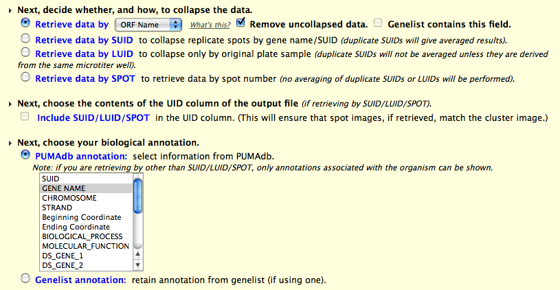
In the example above we have selected experiments from a yeast (SC)
print, and have chosen to collapse and average the data by ORF Name.
This will group and average all the suids for each ORF Name into a
single row in the PCL file. If there are any remaining suids which do
not map to ORF Names, you have the option of discarding them or
retaining them. Each collapsed ORF Name will list the number of suids
it represents in the annotation column of the PCL file. The checkbox
"Genelist contains this field" is used only if you have selected
"Genelist" in the prior step, instead of "All". If the genelist in
this example contained ORF Name, you will need to check the box to
indicate that equality. Note: if you
average by "gene" then you will not be able to create spot images
during the next step in the pipeline. Retrieval of additional
biological annotation is described below.
- Choose the contents of the UID column of the output
file
If you like, you can label each row of data with the Sequence ID
(SUID), the laboratory's microtiter well ID (LUID) and the spot
identifier (SPOT). This information will be produced in your output
preclustering file. For more information, see the File Format Help page. This option
is not available if you are collapsing by gene (see above).
- Selecting biological
annotation
Annotations can be contatenated within the second column of your
retrieved results. Available annotations will vary, depending on the
organism whose sample is being assayed. In the example above, "GENE
NAME" is selected. You can select multiple types of biological data from the multiple-select menu or
you may check the retain annotation from genelist
(if using one) button if you are using your own precompiled
list of genes. For organism-specific details, please refer to the meta-data
for your organism and the Organism Annotation Tables within the database schema. Note: If you are collapsing by "gene" (see above), requests for individual reporter-specific
annotations (oligo sequence, tiling coordinates, sequence description)
are ignored.
- Choose a label for each
array/hybridization
You can label each hybridized array with either the experiment name or
the slide name in the the output preclustering
file. For more information, see the File
Format Help page.
This section of the tool allows you to choose what data you think is
reliable enough to include in your analysis. The steps are:
- Choose the data column to
retrieve
You can select any measurement produced by the feature extraction
software used to analyze the arrays. Different options will be
presented depending on the software used (e.g., GenePix versus
Affymetrix MAS 5). Any field may be used for clustering, but the
defaults presented generally make the most sense. Note that some
fields presented as options may be invalid: e.g., ScanAlyze and
GenePix data are stored together and the same options are presented,
but ScanAlyze and older versions of GenePix do not produce all of the
measurements shown. If no data are retrieved for a given gene (spot,
clone, etc.), either for this reason or because the data are bad or
non-existant for that clone, it will not appear in the final .pcl file
even if you specifically requested data for it in the gene selection
step, above.
- Decide whether to filter by spot flag
Sometimes a spot may be flagged as unreliable, either by software or
based on visual inspection by the experimenter. If a spot has NOT been
flagged, its flag value is 0. If you do not want to retrieve spots
that have been flagged as unreliable, simply keep the default
selection.
- Decide how to handle reverse-dye experiments
This only shows up if you use experiments denoted as reverse. It
inverts ratio and log ratio data properly. If you cluster the
resulting data, the appearance will change and the experiments may
cluster differently, but the gene clustering won't be affected (just
due to the mathematics involved).
- Select criteria for spots to be selected
You can choose to filter out datapoints based on multiple criteria
using these filters. You can combine these filters in several
possible ways using filter strings. Each filter has a checkbox to make
it active or inactive. Check this box if you want to use the filter.
The first pull-down menus indicate which measurement or data point you want
to use in the filter. Remember that not all measurements are
available for hybridizations that were scanned with ScanAlyze instead
of GenePix, or older versions of GenePix. The second pull-down menu
gives you several mathematical operators you can use on your
measurements. The final section you can edit to indicate the value to
which you want to compare your measurements. Several default examples
are available, but you should change the filters as you see fit.
If you don't want your filters joined by "AND"s, use the FilterString box to enter the method by which you want your
filters joined. If you do not enter a filter string, the default is
that all active filters will be connected with the AND operator.
You may enter a string that dictates how you want the
filters combined. For instance, the filter string:
1 AND (2 OR 3)
means that you want datapoints that pass filter 1 and either
filter 2 OR filter 3. (Note: filters 1, 2, and 3 must all
be active for this to work.)
You may also use more complex queries, such as:
(1 AND ((2 OR 3) AND (4 OR 5))) OR 6
The filtering will abort with an error message if the parentheses
don't match or if the string is not
syntactically correct.
- Special note regarding Agilent file formats
Beginning in version 10.5 of the Agilent Feature Extraction software, the default output format is "compact"
which cuts the file size (of the .txt file) by about half. Where the "full" output contains 114
FEATURE attributes, the "compact" only contains 42 (See full and
compact attribute lists). If you load experiments in "compact" version,
be aware that you can only filter by the fields that the compact format supports. (We do no require nor
even recommend that you use the "compact" format. File size is not an
issue for PUMA. To change the setting in the Feature Extraction software,
click the project properties, and select full in the FeatureExtractor output package box.)
- Decide whether to collapse and average experiments from replicate sets, if applicable.
If you have selected experiments that belong to an experiment set which has been designated as a replicate, this option is
available. It allows you to collapse the experiments from the replicate set into a single column whose value is calculated
as either the mean (default) or the median. The title of the resulting column is the name of the experiment set, along with an
asterisk to serve as an indicator that it is an averaged value. Note that if the experiments you chose belong to more than one
replicate set, this option is not available. There is help for creating replicate experiment sets.
- Decide on some image presentation
options
If you are planning on viewing an assembled image of each array,
select the retrieve spot coordinates option.
If you are retrieving a large number of arrays, you are best served by
NOT using this option, since you might run out of memory. The show all spots option allows you to view even the
spots that you filtered out, but can make data retrieval extremely slow.
There are several steps to this part of the tool. Which options
appear depends on what sort of data you have retrieved. Operations
are carried out in the order in which they are presented on the page.
The steps are:
- Choose options for transformation of
single-channel data
These options are available only for single channel data, including
single-channel intensities from two-color arrays. You may choose to
adjust the average values of the retrieved data by multiplying each
value by a constant factor (each array will have a constant calculated
for it specifically). This is essentially a simple cross-array
normalization. Second, you may choose to log-transform the data, with
or without addition of a constant for variance stabilization. This is
generally appropriate if you intend to cluster the data.
- Choose one of these methods to filter
genes based on data distribution
filter genes based on the disribution of their data, leave the "Do not
filter genes on the basis of data distribution" option selected.
Otherwise, you can choose one of two options.
You can use the Rank filter to select only
those genes whose values (log(base2)R/G normalized ratio) are in the
top percentile. You can decide what the percentile must be and the
number of arrays for which a gene must be in your percentile. If you
elect to show the percentiles in your preclustering file (for more
information, see the File Format Help
page), you will be unable to cluster your data with our tools.
You can use the Deviations filters to select
only those genes with a retrieved value different from the mean (for a
single array) by more than a selected multiple of the standard
deviation (for that array). You can decide what that multiple is and
over how many arrays it must be true.
- Decide whether to center data
This option is only available if you are retrieving log-transformed
data. Centering is a data transformation that adjusts the values of
your data. If, for example, you choose to center genes by means, the
mean value for each gene will become zero after the centering. You
can decide whether you want to center genes and/or arrays by either
means or by medians. The mean or median of all values, for each gene
or array, is subtracted from each value for that gene or array.
Centering data for each gene is usually done in those cases where you
are comparing hybridized arrays that use a common reference in the
green channel.
When you choose to center both by gene and by array, you can decide
whether or not to iterate the operation. Upon centering arrays, values
for centered genes may be thrown off, because of missing values, or
when centering by medians. Iterating allows the centering to be
repeated on both genes and arrays until the values stop changing.
Obviously, iterating will increase the time spent calculating your
results. Iteration continues until the maximum change to any array is
less than 0.01 (in units of log-ratio), up to a maximum of ten
iterations.
- Select a method to filter genes based on
data values
These filters are available only if you are retrieving log-transformed
data. You can choose not to filter genes based on their data values,
but if you do, there are two options. The first is to use a Cutoff value, to require values to exceed a given
value for some number of arrays. The mathematical operator to use for
comparison and the value to which the gene's log ratio is being
compared are determined by you. The default setting selects genes
which are at least 4 fold induced or 4 fold repressed in at least 1
experiment. (Note that it is 4 fold, because it is the absolute
log(base2) ratio that must be greater than 2, and thus the
ratio must greater than 4 fold up or down (2^2).) You may change these
settings to suit your needs. For example, you may filter out genes
that vary by this amount in fewer than 3 experiments, or you can
choose ones that vary by a different amount.
If you are retrieving log-transformed ratio data, you can also select
only those genes whose distance in result-space
exceeds a given value. The log transformed data for a given gene
across the selected experiments constitute a vector, and this filter
determines whether the length of this vector is greater than the
specified minimum.
- Choose whether to filter genes and
arrays based on the amount of data passing the spot filter criteria
Based on the filtering criteria you entered in the Select criteria for spots to be selected in the Data Filtering Options section of this
tool, you can now indicate which genes or arrays to use. You can
enter a percentage of arrays for which any gene must pass your filter
criteria. In addition, you can select only those arrays that have
some percentage of spots passing your filter criteria. For example,
if a gene passes your filter in more than 80% of the hybridized arrays
you are analyzing, you will retrieve data for that gene, but only the
data that passes your filter criteria. The data that doesn't pass
will be discarded. If you selected non-log transformed data earlier,
this is the only option available for you to filter the data.
Once
you've submitted a clustering query, you will see a page where text
writes to your screen. When the preclustering file is complete, the
last line will read, "...genes were selected."
- 'Download
Preclustering File' allows you to download the raw data to your
machine for analysis using your own methods.
- 'Clustering and
Image Generation' allows you to view the results after setting some
final clustering option and image generation options.
PUMAdb allows you to perform some
data
analysis on your preclustering file, using either of two methods:
You have to define the following options when hierarchically
clustering
- Whether to cluster genes, and if so whether to use a centered,
or a non-centered metric.
The centered vs non-centered metric only applies if you are using
the Pearson Correlation (see below). It will not make a difference if
using the Euclidean distance.
- Whether to cluster experiments
The same considerations apply for experiments as described for
genes above.
- Whether to use the Pearson Correlation or the Euclidean distance
These are distance
metrics that are used for measuring the similarity of expression
between genes.
- Whether to Hierarchically
Cluster, or make a Self
Organizing Map.
If you choose 'Self Organizing Map Cluster', be sure to specify x
and y dimensions. Your settings for hierarchical clustering
described above will still be used when each partition of the SOM is
clustered.
If you want to generate a file of sorted correlations, the default
correlation is .8. Click 'Submit' when you have chosen the
appropriate options.
Here are a couple tips that will help you optimize the time it takes
to analyze the experiments you selected.
- Selecting 'Show spot images' will slow down the analysis.
- Broken up images load faster and can be navigated more quickly
than unbroken images.
To interactively browse the clustered data, click the red and green
image in the lower left-hand corner of the window. This takes you to
the 'Hierarchical Cluster View' where you can focus on specific gene
sub-clusters.
- The map on the left contains the entire cluster, and
its size can be changed by entering new parameters in the upper
left-hand corner.
- Clicking on this map changes the view of the
graph on the right, which contains the experiment names as
columns and gene names as rows.
You can view the clustered data in the following ways.
- 'View broken images' displays a .gif of the clustered
genes based on the average retrieved value.
- 'View broken spot images'
displays a .gif of the clustered genes. The spots of the experiment
are displayed in a way that allows you to see the variation within
the spot.
- 'View joint broken images' places both the above .gifs in the
same window. If you don't see the broken spot image,
scroll left to bring it onto your screen.
- Clicking on 'pcl' at the bottom of the screen allows you view the
preclustering file.
The other links at the bottom of the screen download files to your
machine.
- 'cdt' downloads the complete tree view datafile.
- 'gtr' downloads the genetree view datafile, which describes the
tree of clustered genes.
- If you chose an experiment clustering option on the previous page,
you will also have the option to click on 'atr' to download the
arraytree file.
