
PUMAdb : Singular Value Decomposition Help
Your session is inactive. Login
Contents
- Description
- SVD tools
- SVD Display
- Classification
- How SVD works
- Multiplying Matrices
- Some Useful References
Related Help Documents
- Repository Help: Explanation of PUMAdb's system to allow you to save and share files at different stages of analysis
- File Formats: Information about preclustering (.pcl), clustered data table (.cdt), gene tree (.gtr) and array tree (.atr) files generated in the process of clustering data
The default column of data that is selected for data retrieval is the Log(base2) of R/G Normalized Ratio (Mean). You may also want to try the R/G Normalized Ratio (Mean), which has not been log transformed.
SVD cannot be performed on datasets with missing data. Therefore, you may want to specify a criteria for spot selection that is somewhat more permissive than the criteria you use when analyzing your data with hierarchical clustering alone, although you should not relax those criteria to the extent that you end up analyzing unreliable data.
You can use SVD by clicking on the "SVD" button for any .pcl file in your repository. There are help documents provided for both the repository and file formats.
In order to use SVD as it is implemented in the context of the database, you will have to first put a preclustering (.pcl) file in your repository. Although the SVD of a dataset is independent of the order of the genes and arrays in the data, a meaningful order might help you correlate dominant eigengenes with experimental artifacts that are superimposed on the data or with biological processes that are present within the data. For this reason, it is often advantageous to order your arrays by using an experiment set or array list (as one might already have done for a time series) or by clustering genes and/or arrays using the database clustering pipeline and then retrieving the data using that order.
Centering your data around the gene average expression is mathematically equivalent to filtering out an eigengene whose expression is constant across all arrays. The ability to do this depends upon obtaining such an eigengene in the decomposition. Deciding whether to center your data prior to using SVD will depend on your experiment. If your data would be appropriately centered prior to clustering (for example, if you are clustering data from a survey of tumor types in comparison to a common reference), then you'll probably want to center the data, cluster and perform SVD on the .pcl file. If your experiment should not be centered (for example, if you are using a biologically meaningful control reference, such as time zero), then don't center prior to clustering or SVD. Usually, SVD of a non-centered dataset indeed results in an almost constant eigengene being the most dominant eigengene in the data. In these cases, SVD of the non-centered data provides some justification for centering the data. Also, SVD of the non-centered dataset will give very similar results to that of the centered dataset, the main difference being that in the decomposition of the non-centered dataset the almost constant eigengene is one of the most significant eigengenes, while in the centered dataset, this eigengene may be one of the least significant eigengenes (compare Figures 1 and 2 below).


Figure 1: Raster Display of
the Eigengenes (Left) and Bar Chart Display of the
![]() Probabilities of Eigenexpression (Right) of Non-Centered Yeast Cell Cycle Data
Probabilities of Eigenexpression (Right) of Non-Centered Yeast Cell Cycle Data


Figure 2: Raster Display of
the Eigengenes (Left) and Bar Chart Display of the
![]() Probabilities of Eigenexpression (Right) of Centered Human Sarcoma Tumor Data
Probabilities of Eigenexpression (Right) of Centered Human Sarcoma Tumor Data
Once a .pcl file has been prepared and saved, you can use SVD by clicking on the "SVD" button in your repository.
Since SVD cannot be performed on datasets with missing values, the first step is to decide whether to discard all genes with missing values or to estimate the values for any data that is missing. Since it is extremely common for a gene to be missing data for at least one array, you may want to replace some of the missing data to retain a larger number of potentially interesting genes. Database software allows you to replace missing data with the value that is the average for all the data for that gene. You can limit the amount of data that can be estimated, so that genes with too much missing data will be discarded from the SVD analysis. Estimated values will not be retained in the resulting .pcl file, so you will not have any "false" data propagated.
The SVD of a dataset is independent of the order of the genes and arrays in the data. However, a meaningful array order may help correlating the dominant eigengenes with experimental artifacts that are superimposed on or biological processes that are manifested in the data. Similarly, a meaningful gene order may help correlating the corresponding eigenarrays with the corresponding cellular states. For time series data, you may want to order the arrays according to the time points that they sample. For tumor data, you may want to cluster both genes and arrays before performing SVD.
The software displays the eigengenes matrix (the left-most matrix in Figure 3) in a red and green raster display alongside a bar chart display of their corresponding probabilities of eigenexpression.

Figure 3: Database tool for viewing and using SVD in gene expression data analysis.
Each row in the Eigengenes Raster Display represents an eigengene pattern of expression. The uppermost row in the eigengenes matrix is the first eigengene, which is the one that contributes the most to the entire dataset. From this display, there are several options that are explained below:
Each row in the bar chart (on the right side of Figure 3) represents the probability of eigenexpression of the corresponding eigengene (and eigenarray). For example, the first (upper most) bar in the chart is the probability of eigenexpression of the first eigengene (and also the first eigenarray). There is more information about probability of eigenexpression and entropy later in this document.
You can view a plot of one or more eigengenes by selecting them using the middle menu ("Select Eigengene(s) to remove or plot"). After highlighting the vector(s) you want to view, just click on the "Plot selected eigengene(s)" button. As illustrated in Figure 4, the next page will present an image much like the one below. You can use this graph to better visualize the eigengenes and to decide whether their patterns appear to be correlated with some underlying biology or an experimental artifact.
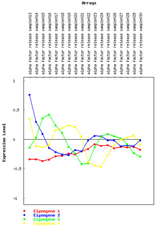
Figure 4: Plot showing the behavior of four eigengenes.
Click on any one of the eigengenes (rows) in the raster display of the eigengenes matrix to display the sorted projections of all genes of your dataset with this eigengene. This display enables you to choose the two subsets of genes from your dataset, with the largest positive or negative projection onto the selected eigengene so that you can analyze them further. This display is illustrated in Figure 5.
Use the "Selecting Subsets of Data" section to select data that you can enter into your repository as a .pcl file or simply download to your desktop computer. Don't forget that you might want to select genes that have high projections in both the positive and negative directions. You can then cluster or further analyze the data for those genes to look for patterns. There is more information about genes' projections later in this document.
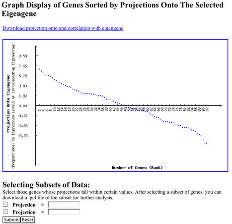
Figure 5: Projection of genes within an eigengene. This image shows how all genes in a dataset are projected onto a given eigengene. This is one way to determine those genes whose expression is significantly contributed to by an eigengene.
Once you have used the "Plot selected eigengene(s)" option and have examined the projection of genes in an eigengene, you may be able to determine that a given eigengene represents experimental artifacts in your data. If you detect an artifact in your experiment, the first thing that you should do is to see whether there is some basis for your artifact. For instance, does the artifact correspond to some experimental parameter, such as the date of hybridization, or the print batch? The best option is to see if the data themselves can be corrected upstream, eg if there is a print batch difference, was there a problem with the print? Do the genes with the greatest projection in the eigengene that represents the artifact come from a limited number of microtiter plates? In the case that you have an artifactual pattern in your data, that confounds your analysis of the data, and you are unable to remove it upstream, then it is likely that you want to somehow remove that pattern. One method to do this would be to separately center the two groups of arrays that exhibit the artifact differentially, and then to recombine the data. If the artifact is expected to affect each array within the two groups equally, this is probably the most appropriate method to deal with the artifact. On the other hand, if an artifact is not likely to affect arrays equally, eg cells experienced some heat shock at the beginning of an experiment, and this effect is reduced over time, but not really part of the experiment, then a corresponding eigen gene can be removed by SVD. You can do this by highlighting the eigengene(s) you wish to remove and clicking on the "Remove selected eigengene(s)" option. The new dataset can be further examined using SVD or can be saved as a .pcl file for clustering or other analyses.
Removing an eigengene is mathemetically equivalent to setting the eigenexpression level of this eigengene (and at the same time, its corresponding eigenarray) to zero. The three matrices (the eigenarrays matrix, the eigenexpression matrix and the eigengene matrix) are then mulitplied again to reconstruct a microarray dataset with the effects of the eigengene (and its corresponding eigenarray) removed.
After removing an eigengene, the genes and arrays that were in the original microarray dataset are still there, but the expression data itself has changed. For example, a gene that had most of its contribution from a filtered eigengene would appear to have an almost constant zero expression across all the arrays. Since data values are now changed, if filters based on data values are important to your analysis, you might want to re-filter your reconstructed data.
After removing any eigengenes that represent experimental artifact and clustering, you may want to use SVD again. By sorting the genes by their projections onto eigengenes of interest, you can identify genes that might be involved in a given biological process.
In order to do this, you may want to further examine the dominant eigengenes of your dataset (and the corresponding eigenarrays). Sometimes, an eigengene (and its corresponding eigenarray) that is not highly significant will still be very interesting due to its expression pattern. If you construct different datasets from your data (for example, by using different parameters to select or filter genes and arrays) you may want to try SVD on all your datasets. Any eigengene that appears to be of a similar expression pattern with a similar probability of eigenexpression in the decompositions of all of these datasets is a robust eigengene that may be reflecting an interesting biological process.
Once you are satisfied that one or more eigengenes in the SVD of your data represent biological processes of interest, you may classify the genes and arrays according to their expression in this subset of eigengenes and eigenarrays, rather than by their overall expression. Of course, you already sorted the genes based on either their projection onto or their correlation with each of these eigengenes, to satisfy yourself that they capture some biology. Note that you can also sort the arrays based on their projection onto each of these eigenarrays, by sorting the arrays according to their expression in each of the corresponding eigengenes separately.
The goal of SVD is to find a set of patterns that describe the greatest amount of variance in a dataset. A simple way to conceptualize how to do this is to think about how to represent a cigar in two dimensions. Take a look at Figure 6A and try to decide what "shadow" provides the greatest amount of information about our cigar.
Figure 6: Schematic (and mathematically inaccurate!) representation of how SVD finds the "view" of data that captures the greatest variance.
The shadow that shows the length of the cigar (Figure 6B) would give us the most information about the shape of the cigar. Now if we took another shadow, one orthogonal (perpendicular or 90 degrees away) to the one showing the length of the cigar, the most meaningful shadow would be that showing the width of the cigar (Figure 6C). SVD attempts to do something very similar. First, it finds a pattern that accounts for the greatest amount of variance in the data (in the case of our cigar, it would be the long shadow in Figure 6B). The next pattern is one that is orthogonal to the first and accounts for the next highest amount of variance (for example, Figure 6C). Each pattern is orthogonal to the others and accounts for a decreasing amount of the variance in the data.
Singular value decomposition (SVD) is a data-driven mathematical framework for the description of genome-scale expression data, where both the mathematical variables and operations may represent some experimental or biological reality, as is described in Alter et al. (and see also http://genome-www.stanford.edu/SVD/). In these cases, the mathematical variables of SVD are useful in extracting biological information from the data. And, the mathematical operations of SVD are useful in manipulating the data.
Usually, SVD gives a unique decomposition of the data. This means that for each dataset there exists only one set of eigengenes, eigenexpression levels and eigenarrays, that satisfies the mathematical requirements of SVD. Note that mathematically, each eigengene and eigenarray is defined up to a factor of ±1. This means that each eigengene and eigenarray capture both parallel and antiparallel gene and array expression patterns, respectively. However, when the eigenexpression levels of a group of eigengenes (and eigenarrays) are almost equal, the decomposition is not unique. In such cases, this group of eigengenes and eigenarrays that are given by the numerical computation of SVD, most likely do not correspond to any independent processes or cellular states, which are manifest in the data.
Dominant eigengenes may capture expression patterns that are correlated with experimental artifacts. For example, an eigengene pattern may be correlated with variations in (a) the day of hybridization (as is described in Alter et al.), (b) array print size (as is described in Nielsen et al.), or (c) scanner calibration (as is described in Bohen et al.). In general, any significant variation in the experimental protocol that is used in the collection of the data among the arrays in a dataset may be represented by one or more eigengenes. The eigenarrays, in these cases, represent the genome-scale effects of these artifacts.
These artifacts can then be removed from the overall expression data (without discarding the data for any of the genes or arrays) by filtering out the corresponding eigengene(s) and eigenarray(s). This SVD data normalization, where additive and possibly also multiplicative experimental artifacts are being detected and filtered out, enables better further analysis with methods such as hierarchical clustering, which are sensitive to the presence of an artifact that is superimposed on the data.
The eigengenes may also capture expression patterns that are correlated with some of the independent regulatory programs or biological pathways which are manifest in the dataset. The eigenarrays, in these cases, capture the corresponding cellular states. For example, eigengene and eigenarray patterns may be correlated with (a) the observed genome-wide effect of a known regulator, and the measured sample in which this regulator is overactive (as is described in Alter et al.), or (b) a group of genes that are differentially expressed among a set of tumor samples, and the corresponding classification of these samples, respectively (as is described in Nielsen et al.).
The genes and arrays can then be classified according to their expression in this subset of eigengenes and eigenarrays, rather than by their overall expression. Note that this SVD classification allows each gene and array to be in more than one category of classification. This SVD classification is usually also more robust than other classification methods, such as hierarchical clustering, where the classification is according to the overall expression pattern of each gene and array. This is because SVD classification is usually less sensitive to artifacts that may be superimposed on the data or to variations in the genes and arrays that are selected to make up the dataset.
SVD is a linear transformation that uses a theorem from linear algebra to decompose a matrix to the product of three other matrices. For microarray data, the mathematical variables of SVD are the "eigengenes," "eigenarrays" and "eigenexpression levels." The eigengenes are gene patterns of expression (the shadows of the cigar). The eigenarrays are array patterns of expression. And, the eigenexpression levels indicate the dominance, and therefore also the significance, of these gene and array patterns of expression in the data. These matrices are shown in Figure 7:
Figure 7: Singular value decomposition of a matrix of gene expression values (matrix A) results in three matrices, U (the eigenarrays matrix), W (the eigenexpression levels matrix) and VT (the eigengenes matrix). Matrix VT contains the eigengenes, matrix W contains the eigenvalues, matrix U contains the coefficients for the genes for each eigengene.
Let us assume that we have a matrix named A of gene expression data, where the number of genes is M and the number of arrays is N. SVD will decompose our matrix A into three matrices, which will re-construct matrix A when multiplied together (there is a brief refresher on matrix multiplication in this document):
A = U x W x VT
Two more examples of this are shown below:
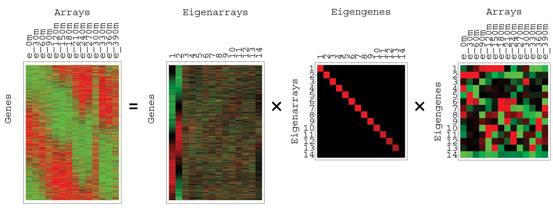
Figure 8: SVD of Yeast Cell Cycle
Data
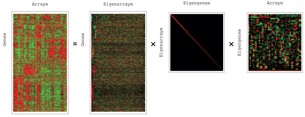
Figure 9: SVD of Human Sarcoma
Tumor Data
The data expression matrix tabulates the expression of both genes and arrays: The rows of the data expression matrix tabulate the expression of each gene in the dataset across all arrays, and the columns – the expression of each array across all genes.
The EigenarraysThe U matrix in the above example is also called the eigenarrays matrix and has NxM dimensions. Each column is an eigenarray, which reflects the decomposition of the data for the arrays across all genes. The first column in the eigenarrays matrix is the first eigenarray, or rather the pattern that captures the most information across all genes. All the eigenarrays are orthogonal to one another and are therefore completely uncorrelated. Each eigenarray is normalized to have a vector size of one.
Within the framework of SVD, the expression of each array is a superposition (or a weighted sum) of all of the eigenarrays. Therefore, SVD separates the expression of each array into the uncorrelated contributions of all the of eigenarrays. Note that these contributions may be positive as well as negative.
The Eigenexpression LevelsThe W matrix has NxN dimensions and is called the Eigenexpression Levels matrix. Each entry records the expression of an eigengene in an eigenarray. In other words, it provides a coefficient for the role an eigengene plays in an eigenarray (and vice-versa). The first entry in the eigenexpression levels matrix records the level of expression of the first eigengene in the first eigenarray.
The eigenexpression levels matrix is always diagonal. This means that each eigengene is expressed only in the corresponding eigenarray, with the corresponding eigenexpression level. The eigenexpression levels are always nonnegative (larger than or equal to zero). They are always arranged in decreasing order. This means, for example, that the eigenexpression level of the first eigengene and eigenarray is always higher than or equal to the eigenexpression level of the second eigengene and eigenarray.
Each eigenexpression level represents the dominance of the corresponding eigengene and eigenarray: The higher is the eigenexpression level, the more dominant are these eigengene and eigenarray in the data. This means, for example, that the first eigengene and eigenarray are always more dominant than or as equally dominant as the second eigengene and eigenarray.
Eigen ProbabilitiesThe probabilities of eigenexpression that are presented in this bar chart are calculated from the eigenexpression levels that appear in the diagonal matrix of the SVD of the dataset (see Figure 8). The probability of eigenexpression indicates the significance of an eigengene and its corresponding eigenarray in terms of the fraction of the overall expression information that they capture in the dataset. It can be thought of as the probability that this eigengene pattern is manifest as a component of the expression of any one of the genes. At the same time it can also be thought of as the probability that the corresponding eigenarray pattern is manifest as a component of the expression of any one of the arrays. Probabilities are calculated by dividing the square of the lth eigenvalue (from matrix W) by the sum of the squares of all the eigenvalues and they are shown as a red bar graph at the right in Figure 1.
Usually, SVD gives a unique decomposition of the data. This means that for each dataset there exists only one set of eigengenes, eigenexpression levels and eigenarrays, that satisfies the mathematical requirements of SVD. Note that each eigengene and eigenarray capture both parallel and antiparallel gene and array expression patterns, respectively. However, when the eigenexpression levels of a group of eigengenes (and eigenarrays) are almost equal, the decomposition is not unique. In such cases, this group of eigengenes and eigenarrays that are given by the numerical computation of SVD most likely do not correspond to any independent processes or cellular states.
Software presents the "entropy" of the dataset in the caption of the bar chart (eg see Figures 1-3 above). The entropy of the dataset measures the complexity of the data from the distribution of the overall expression among the different eigengenes and corresponding eigenarrays, and is calculated from the probabilities of eigenexpression of the dataset. The entropy of an ordered and redundant dataset, in which all expression is captured by a single eigengene and its corresponding eigenarray, is 1. The entropy of a disordered and random dataset, where all eigengenes and eigenarrays are equally expressed, is 0. Usually, the entropy of a non-centered expression dataset is about 0.1 – 0.3, and the entropy of a centered expression dataset is about 0.75 – 0.95. Filtering eigengene and eigenarray patterns out of the dataset will change the entropy of the dataset.
The Eigengenes
VT, or the eigengenes matrix, is an
NxN matrix of eigengenes across all
arrays. Eigengenes are analogous to the shadows of our cigar. The
uppermost row in the eigengenes matrix is the first eigengene, or
rather the one that records a pattern that is shared by the largest
numbers of genes. As with the eigenarrays matrix, the eigengenes are
always orthogonal to one another and are arranged in decreasing order
of dominance.
The last of the three matrices generated by SVD is the matrix
U. There are M rows containing data for
genes in the original dataset (the first row corresponds to the first
gene in the dataset, the second row corresponds to the second gene in
the dataset, etc.). Each column represents an eigen array (the first
column corresponds to the first eigengene, the second column
corresponds to the second eigengene, etc.). Each cell in the
matrix gives the coefficient by which the product of W x
VT should be multiplied to get the amount
that the eigengene contributes to the data vector for that gene.
Which is really just the long way to restate that our original dataset
can be represented as:
A = U x W x
VT
Within the framework of SVD, the expression of each gene is a
superposition (or a weighted sum) of all of the eigengenes. Therefore,
SVD separates the expression of each gene into the uncorrelated
contributions of all the eigengenes. Note that these contributions may
be positive as well as negative.
What Does Superposition of Expression Data
Mean?
Within the framework of SVD, the expression of each gene and array is
a superposition (or a weighted sum) of all of the eigengenes and
eigenarrays, respectively. You could think of the SVD's mathematical
separation of the expression patterns of the genes and arrays into
eigengenes and corresponding eigenarrays, respectively, as attempting
to unravel the overall expression signal into its generating
components: independent experimental and biological processes, and the
corresponding cellular states. In other words, SVD can be used to
attempt to describe expression data as the outcome of a simple
network, where a few independent sources of expression, experimental
or biological, affect all the genes in the dataset (Figure 10). Classification of genes and arrays using hierarchical clustering
results in groups of genes of similar contributions from all the
different sources of expression. You may be interested, however, in
grouping genes according to the effects of only a subset of the
different sources of expression. For example, when one of the sources
is an experimental artifact, you may not want the contribution of this
artifact to influence the classification of the genes. On the other
hand, if one of the sources is due to a pathway of interest, you may
want to isolate the effect of this pathway from that of all other
pathways that give rise to the overall expression data. In these
cases, SVD may be able to aid the analysis of your data by providing
you with the mathematical framework to represent different processes
that affect your data.
Genes' Projections Onto and Correlations With
Selected Eigengene.
The contribution of an eigengene to the overall expression of a
gene is "the projection of the gene onto the eigengene" (Figure
8). This projection may be positive as well as negative, which means
that the contribution of an eigengene to the overall expression of a
gene may be parallel as well as antiparallel to the expression pattern
of the eigengene. Therefore, you would want to see whether there
exists a coherent biological theme reflected in the annotations of the
genes, with the largest positive projections onto the eigengene
(largest parallel contributions from the eigengene). And you would
also want to see whether there exists a separate coherent biological
theme reflected in the annotations of the genes with the largest
negative projections (largest antiparallel contributions from this
eigengene).
Note that the projection of a gene onto an eigengene relative to that
of another gene is listed in the eigenarray which corresponds to this
eigengene. This means that the projection of all genes in the dataset
onto an eigengene are linearly proportional to the corresponding
eigenarray.
The similarity of a gene's expression pattern to the eigengene's
expression pattern is measured by "the gene's correlation with the
eigengene" (Figure 11). You can think of this correlation in
geometrical terms as the cosine of the angle between the gene and the
eigengene, each representing a vector in space. Again, you would want
to see whether there exists a coherent biological theme reflected in
the annotations of the genes, with the largest positive correlations
with the eigengene (with the patterns most similar to that of the
eigengene). And you would also want to see whether there exists a
separate coherent biological theme reflected in the annotations of the
genes with the largest negative correlations (with the patterns most
similar to the patterns that is antiparallel to that of the
eigengene).
The projection and correlation are complementary measures for the
relation between the expression patterns of a gene and an
eigengene. For example, a gene may have a very large projection onto
an eigengene and a very low correlation with this eigengene at the
same time. This may be the case for genes with large expression
variation across the arrays in the dataset: their projections onto all
other eigengenes may be even larger than their projections onto the
eigengene of interest, resulting with low correlations with this
eigengene. Also, a gene may have a relatively small projection onto an
eigengene and yet a very high correlation with this eigengene. This
may be the case for genes whose expression patterns are of small
amplitudes, yet they are almost parallel or antiparallel to that of
the eigengene.
The SVD analysis tools within the database are based on:
The mathematics and computation of SVD are described in: 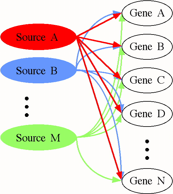
Figure 10: SVD can be used in an
attempt to describe the expression data as the outcome of a network of
processes. Each "source" represents a process (either biological or
artifactual) that has an effect on the expression of each gene. The
effect of any process can be large or small, positive or negative.
Figure 11: Geometrical
Description of a Gene's Projection Onto and Correlation With an
EigengeneMultiplying Matrices
For those who haven't had to multiply matrices since high school, here
is a very brief refresher that might help you understand how your
original dataset relates to the three matrices generated by SVD. When
we multiply the two matrices below, we get a 2 by 2 matrix as follows:
A B C      G H      (AG + BI + CK) (AH + BJ + CL)
D E F   X  I J  =   (DG + EI + FK) (DH + EJ + FL)
           K L
We can do the same type of operation with numbers, as illustrated below:
1 2 3      1 2     (1 + 6 + 15)  (2 + 8 + 18)      22 28
4 5 6   x  3 4  =  (4 + 15 + 30) (8 + 20 + 36)  =  49 64
           5 6
When we multiply the three matrices below, we get a 3 by 2 matrix as
follows:
a b      m 0      g h     (agm+bin) (ahm+bjn)
c d   x  0 n   x  i j  =  (cgm+din) (chm+djn)
e f                       (egm+fin) (ehm+fjn)
And with numbers:
1 2      1 0      1 2     13 18
3 4   x  0 2   x  3 4  =  27 38
5 6                       41 58
References
Alter, O.,
Brown, P. O. and Botstein, D. (2000) Proc. Natl. Acad. Sci. USA
97, 10101
(supplemental material at
http://genome-www.stanford.edu/SVD/).
Golub, G. H. and Van Loan, C. F. (1996) Matrix Computation, 3rd
ed. (Johns Hopkins University Press, Baltimore).